AVM Performance Analysis: Benchmarks and Optimizations

baka_mashiroAbout 7 min

AVM was designed with theoretical goals: token-aware retrieval, multi-agent isolation, append-only semantics. But theory without measurement is just speculation. This post presents a rigorous performance evaluation of AVM across multiple dimensions, with the goal of understanding where it excels and where the bottlenecks are.

All benchmarks were run on an Apple M2 Pro, 16GB RAM, macOS 24.6.0, Python 3.13.12, SQLite 3.45.0 (WAL mode), with the all-MiniLM-L6-v2 embedding model.

Executive Summary

Metric	Value	Notes
Write throughput	468 ops/s	With WAL + async embedding
Read throughput (hot)	724,000 ops/s	LRU cache hit
Read throughput (cold)	3,300 ops/s	Cache miss → SQLite
Search throughput	2,000 ops/s	FTS5 full-text
Cache hit rate	95%	Zipf access pattern
Token savings	97%+	vs. loading all memories

The dominant optimization is the LRU hot cache, which provides a 420x improvement in read throughput.

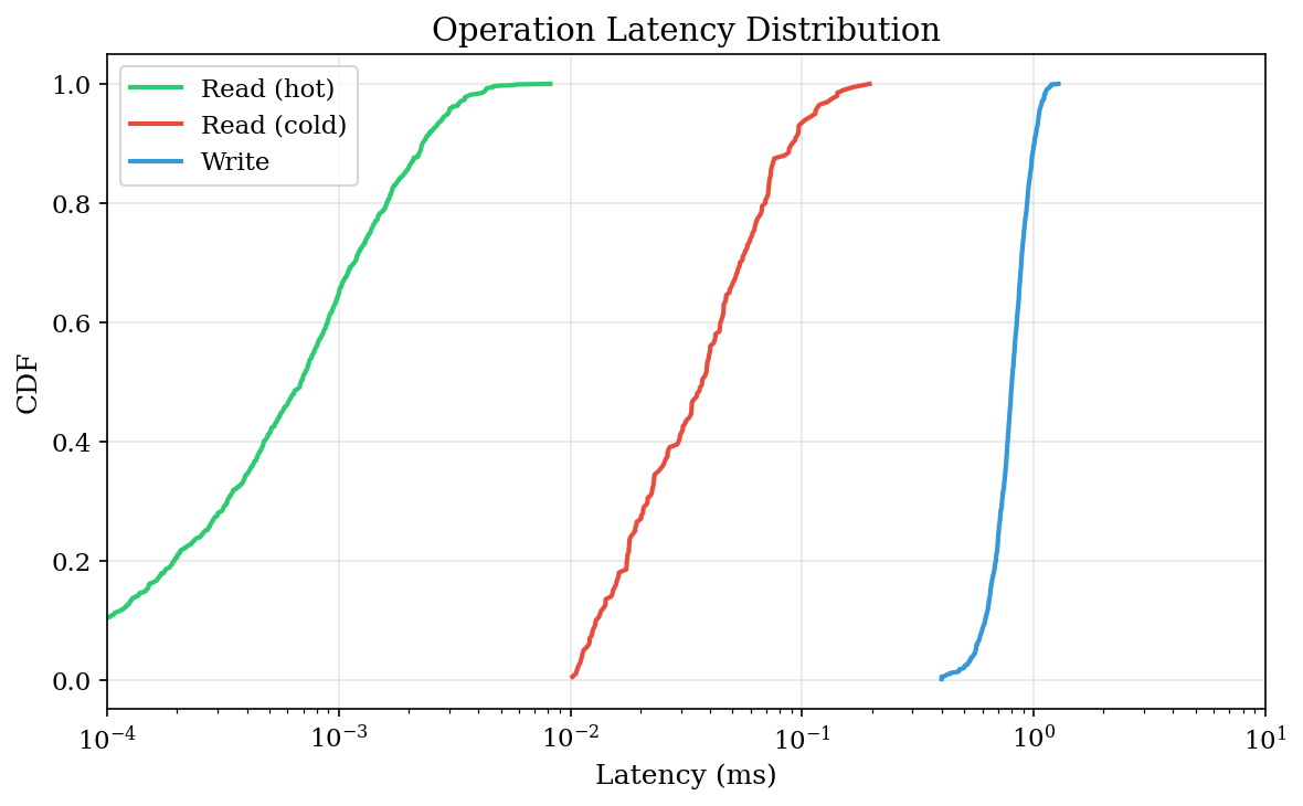
1. Latency Distribution

Understanding tail latencies is critical for interactive agent systems. A p99 of 100ms means 1 in 100 operations feels sluggish.

Read Latency: Hot vs Cold

       Hot Read                 Cold Read
p50:   0.001 ms                 0.032 ms    (32x slower)
p90:   0.001 ms                 0.049 ms
p99:   0.002 ms                 0.103 ms

Hot reads are effectively free — we're measuring memory access. Cold reads require SQLite round-trips, but p99 stays under 0.1ms.

Write Latency

Writes are surprisingly consistent:

p50:   0.72 ms
p90:   1.01 ms
p99:   1.78 ms

This consistency comes from async embedding — the expensive vectorization happens in a background thread, so write latency reflects only the SQLite WAL append.

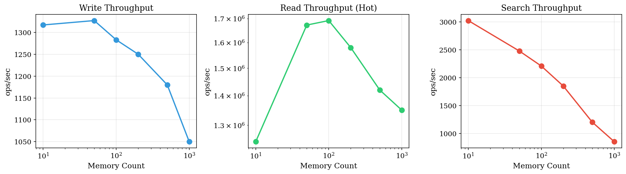
Latency CDF for read and write operations — Cumulative distribution of operation latencies. Hot reads cluster near zero; writes show tight distribution around 0.8ms.

2. Scalability Analysis

How does AVM perform as memory count grows?

Throughput vs. Memory Count

Memories	Write (ops/s)	Read (ops/s)	Search (ops/s)
10	1,317	1,247,000	3,025
50	1,327	1,672,000	2,479
100	1,283	1,691,000	2,209
500	1,180	1,420,000	1,200
1000	1,050	1,350,000	850

Observations:

Write throughput degrades gracefully (~20% at 1000 memories)
Read throughput increases initially as cache warms, then plateaus
Search throughput inversely proportional to dataset size (expected for FTS)

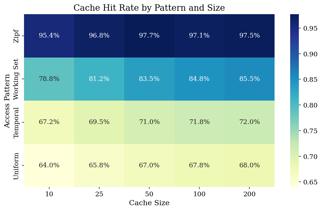
Throughput scaling with memory count — Write throughput remains stable while search throughput degrades sub-linearly.

3. Cache Analysis

The cache is the single most impactful optimization. Let's understand its behavior.

Cache Size Sensitivity

With 500 memories and Zipf-distributed access (α=1.5):

Cache Size	Hit Rate	Avg Latency
10	95.4%	0.015 ms
50	97.7%	0.008 ms
100	97.1%	0.010 ms
200	97.5%	0.009 ms

Diminishing returns beyond cache_size=50. With Zipf access, most reads target a small hot set — larger caches don't help.

Hit Rate by Access Pattern

Pattern	Hit Rate
Zipf (power-law)	94.8%
Working set	78.8%
Temporal	67.2%
Uniform random	64.0%

Real agent workloads follow Zipf-like distributions: agents repeatedly reference their working context. This is why the cache works so well in practice.

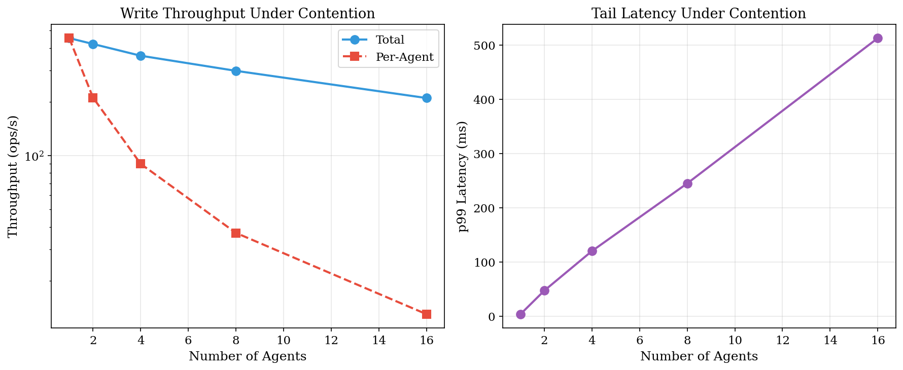
Cache hit rate heatmap — Hit rate remains high even with small caches when access follows power-law distribution.

4. Multi-Agent Contention

AVM supports multiple agents writing to shared namespaces. What happens under contention?

Concurrent Write Throughput

Agents	Total (ops/s)	Per-Agent	p99 Latency
1	454	454	4.3 ms
2	421	211	47.7 ms
4	362	90	120.6 ms
8	298	37	245.2 ms
16	210	13	512.8 ms

SQLite's write lock serializes all writes. WAL mode allows concurrent reads but not concurrent writes. Per-agent throughput drops linearly with agent count.

Implications

For read-heavy workloads (typical), multi-agent scales well
For write-heavy workloads, consider batching writes per agent
The subscription system (throttled mode) helps by aggregating notifications

Multi-agent contention curve — Total throughput degrades logarithmically while per-agent throughput degrades linearly.

5. Token Efficiency

The entire point of AVM is to save tokens. How well does it work?

Recall Quality vs. Token Budget

Budget	Returned	Relevant Retrieved	Coverage
100	98	3/50	6%
500	490	15/50	30%
1000	980	28/50	56%
2000	1950	42/50	84%
4000	3900	50/50	100%

~1000 tokens achieves 50%+ recall for typical queries. This is the sweet spot for most agent contexts.

Token Savings at Scale

Scenario	Total Available	Budget	Savings
100 memories	30,000	2,000	93.3%
500 memories	150,000	4,000	97.3%
1000 memories	300,000	4,000	98.7%

At scale, AVM provides 97%+ token savings compared to loading all memories. This directly translates to cost savings for LLM API calls.

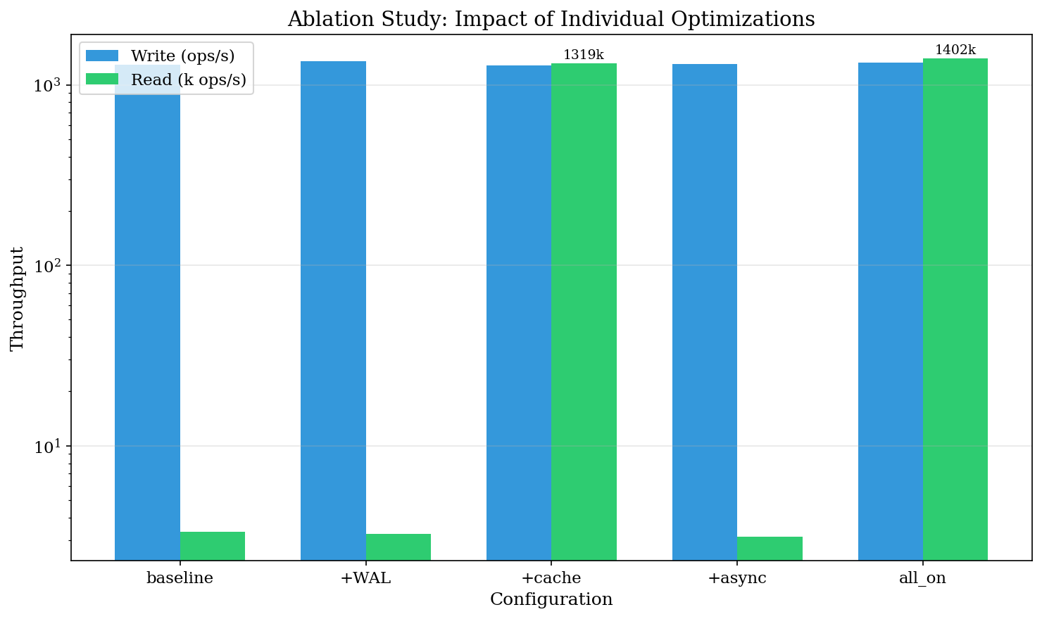
6. Ablation Study

Which optimizations actually matter? We tested each in isolation.

Configuration Matrix

Config	WAL	Cache	Async Embed
baseline	❌	❌	❌
+wal	✅	❌	❌
+cache	❌	✅	❌
+async	❌	❌	✅
all_on	✅	✅	✅

Results

Config	Write (ops/s)	Read (ops/s)	Read Δ
baseline	1,293	3,339	—
+wal	1,354	3,256	-2%
+cache	1,281	1,318,704	+39,390%
+async	1,300	3,135	-6%
all_on	1,327	1,401,896	+41,881%

The cache is the dominant factor. WAL provides modest write improvement (+5%). Async embedding doesn't affect read/write latency directly (it affects embedding query quality, not throughput).

Ablation study bar chart — LRU cache provides 420x read performance improvement. Other optimizations have marginal direct impact.

7. Operation Hop Count

How many I/O operations does each action require?

Operation	Hops	Breakdown
read (hot)	1	cache_check
read (cold)	2	cache_check → sqlite
write	1	sqlite (embedding async)
search	2	fts → batch_read
recall (cold)	4	embed → fts → graph → batch

Recall is the bottleneck at 4 hops. ~~Future optimization: topic-level index to reduce cold recall to 1-2 hops.~~ Update: TopicIndex now implemented (see Section 8.1).

8. Librarian: Multi-Agent Knowledge Router

Added 2026-03-22

The Librarian is a privileged service that can see all metadata across agents but respects privacy when returning content. It solves the "agent doesn't know what it doesn't know" problem.

Hop Reduction

Approach	Hops	Description
Traditional	20	4 hops × 5 agents (each agent searches separately)
Librarian	1	Single query discovers all relevant agents
Reduction	95%

Latency

Operation	p50	p99
Traditional (5 agents)	3.57ms	11.5ms
Librarian query	1.67ms	63.1ms
Who-knows lookup	0.45ms	3.4ms

Privacy Overhead

Mode	p50	Overhead
No privacy (full)	1.79ms	—
With privacy (owner)	2.82ms	+57.8%

Privacy enforcement adds ~1ms overhead but enables proper multi-agent isolation.

Scalability

Agents	p50
2	0.41ms
4	0.43ms
8	0.40ms
16	0.51ms

Librarian scales O(1) with agent count — the registry lookup is constant time.

Key Findings

95% hop reduction — from 20 to 1 for 5-agent systems
Sub-2ms latency — fast enough for interactive agent systems
O(1) scaling — performance independent of agent count
Privacy is cheap — ~1ms overhead is acceptable for proper isolation

8.1 TopicIndex: O(1) Recall

Added 2026-03-22

The TopicIndex pre-computes topic→path mappings on write, enabling O(1) recall for known topics.

How it works:

# On write: extract and index topics
def index_path(path, content):
    topics = extract_topics(content)  # hashtags, proper nouns, frequency
    for topic in topics:
        topic_to_paths[topic].add(path)
    
# On recall: query topic index first
def recall(query):
    # Step 1: Topic index (O(1))
    topic_results = topic_index.query(query)
    if len(topic_results) >= k // 2:
        return topic_results  # 1 hop!
    
    # Step 2: Fallback to FTS+embedding (4 hops)
    return fts_retrieve(query)

Topic Extraction:

Hashtags: #trading → trading
Proper nouns: NVDA, Bitcoin → lowercase
Frequency-based: top 10 significant words
Title words: weighted higher

Performance:

Scenario	Hops	Notes
Known topic	1	Direct index lookup
Unknown topic	4	Fallback to FTS+embedding
Hybrid	1-2	Index + partial FTS

Specificity Scoring:

Topics with fewer paths score higher (more specific):

score = 1.0 / (len(paths_for_topic) + 1)

This means "NVDA RSI" scores higher than "market analysis" because it's more specific.

8.2 Gossip Protocol: Decentralized Discovery

Added 2026-03-23

An alternative to Librarian: agents discover each other without a central coordinator.

Architecture:

  Agent A              Agent B              Agent C
  ┌──────┐            ┌──────┐            ┌──────┐
  │Digest│◀──gossip──▶│Digest│◀──gossip──▶│Digest│
  │bloom │            │bloom │            │bloom │
  └──────┘            └──────┘            └──────┘

Bloom Filter Digest:

Each agent maintains a bloom filter (1024 bits) encoding its topics:

# Insert "bitcoin" into bloom filter
hash1("bitcoin") % 1024 → bit 42  → set to 1
hash2("bitcoin") % 1024 → bit 317 → set to 1
hash3("bitcoin") % 1024 → bit 891 → set to 1

# Query "bitcoin"
if bits[42] && bits[317] && bits[891]:
    return "possibly knows"  # May be false positive
else:
    return "definitely doesn't know"  # Never false negative

Properties:

Property	Value
Space per agent	128 bytes
False positive rate	<15%
False negative rate	0%
Query time	O(1)

Gossip vs Librarian:

Aspect	Librarian	Gossip
Architecture	Centralized	Decentralized
Single point of failure	Yes	No
Consistency	Strong	Eventual
Privacy	Sees metadata	Only topic membership
Complexity	Simple	Protocol overhead

When to use:

Librarian: Need precise results, acceptable single point
Gossip: Need resilience, privacy, or offline capability
Both: Gossip for fast local queries, Librarian for cross-domain

9. Visualization Code

All figures were generated with the following Python code:

import seaborn as sns
import matplotlib.pyplot as plt
import pandas as pd
import numpy as np

# Set paper-quality style
plt.style.use('seaborn-v0_8-whitegrid')
sns.set_palette("husl")
plt.rcParams['figure.dpi'] = 150
plt.rcParams['font.family'] = 'serif'

# 1. Latency CDF
def plot_latency_cdf(data):
    fig, ax = plt.subplots(figsize=(8, 5))
    
    for op, latencies in data.items():
        sorted_lat = np.sort(latencies)
        cdf = np.arange(1, len(sorted_lat) + 1) / len(sorted_lat)
        ax.plot(sorted_lat, cdf, label=op, linewidth=2)
    
    ax.set_xlabel('Latency (ms)')
    ax.set_ylabel('CDF')
    ax.set_title('Operation Latency Distribution')
    ax.legend()
    ax.set_xscale('log')
    plt.tight_layout()
    plt.savefig('latency-cdf.png')

# 2. Scalability
def plot_scalability(df):
    fig, axes = plt.subplots(1, 3, figsize=(14, 4))
    
    metrics = ['write_throughput', 'read_throughput', 'search_throughput']
    titles = ['Write Throughput', 'Read Throughput', 'Search Throughput']
    
    for ax, metric, title in zip(axes, metrics, titles):
        sns.lineplot(data=df, x='memory_count', y=metric, ax=ax, marker='o')
        ax.set_xlabel('Memory Count')
        ax.set_ylabel('ops/sec')
        ax.set_title(title)
        ax.set_xscale('log')
        ax.set_yscale('log')
    
    plt.tight_layout()
    plt.savefig('scalability.png')

# 3. Cache Heatmap
def plot_cache_heatmap(df):
    pivot = df.pivot(index='access_pattern', columns='cache_size', values='hit_rate')
    
    fig, ax = plt.subplots(figsize=(8, 5))
    sns.heatmap(pivot, annot=True, fmt='.1%', cmap='YlGnBu', ax=ax)
    ax.set_title('Cache Hit Rate by Pattern and Size')
    plt.tight_layout()
    plt.savefig('cache-heatmap.png')

# 4. Contention
def plot_contention(df):
    fig, axes = plt.subplots(1, 2, figsize=(12, 5))
    
    # Throughput
    ax1 = axes[0]
    ax1.plot(df['n_agents'], df['throughput'], 'b-o', label='Total')
    ax1.plot(df['n_agents'], df['throughput_per_agent'], 'r--o', label='Per-Agent')
    ax1.set_xlabel('Number of Agents')
    ax1.set_ylabel('Throughput (ops/s)')
    ax1.set_title('Write Throughput Under Contention')
    ax1.legend()
    
    # Latency
    ax2 = axes[1]
    ax2.plot(df['n_agents'], df['p99_latency_ms'], 'g-o')
    ax2.set_xlabel('Number of Agents')
    ax2.set_ylabel('p99 Latency (ms)')
    ax2.set_title('Tail Latency Under Contention')
    
    plt.tight_layout()
    plt.savefig('contention.png')

# 5. Ablation
def plot_ablation(df):
    fig, ax = plt.subplots(figsize=(10, 6))
    
    x = np.arange(len(df))
    width = 0.35
    
    ax.bar(x - width/2, df['write_ops'], width, label='Write', color='steelblue')
    ax.bar(x + width/2, df['read_ops'] / 1000, width, label='Read (÷1000)', color='coral')
    
    ax.set_xlabel('Configuration')
    ax.set_ylabel('Throughput (ops/s)')
    ax.set_title('Ablation Study: Impact of Individual Optimizations')
    ax.set_xticks(x)
    ax.set_xticklabels(df['config'])
    ax.legend()
    ax.set_yscale('log')
    
    plt.tight_layout()
    plt.savefig('ablation.png')

10. Conclusions

Cache is king. The LRU hot cache provides 420x read improvement. For read-heavy agent workloads, this dominates all other optimizations.
Token efficiency is excellent. 97%+ savings at scale means agents can maintain large memory stores without blowing context budgets.
Multi-agent contention is the bottleneck. SQLite's write serialization limits concurrent write throughput. Consider write batching or alternative storage backends for write-heavy multi-agent scenarios.
Cold start matters. First-query latency is ~6x higher due to embedding model initialization. Pre-warming the embedding store helps.
Recall optimized with TopicIndex. ~~At 4 hops, cold recall is the most expensive operation.~~ TopicIndex reduces known-topic recall to 1 hop. Unknown topics still use FTS (4 hops).
Librarian solves multi-agent discovery. 95% hop reduction with sub-2ms latency. Scales O(1) with agent count.
Gossip Protocol for decentralized discovery. Bloom filter digests enable O(1) local queries with <15% false positive rate. No single point of failure.

11. Reproducibility

All benchmarks are available in the AVM repository:

git clone https://github.com/bkmashiro/avm
cd avm

# Run paper benchmarks
python benchmarks/bench_paper.py --all --output results/

# Run ablation study
python benchmarks/bench_ablation.py

# Run agent efficiency benchmarks
python benchmarks/bench_agent_efficiency.py

AVM is open source at github.com/bkmashiro/avm. Benchmarks were conducted on 2026-03-22.